Gaussian Processes for Machine Learning by Rasmussen and Williams has become the quintessential book for learning Gaussian Processes. They kindly provide their own software that runs in MATLAB or Octave in order to run GPs. However, I find it easiest to learn by programming on my own, and my language of choice is Python. This is the first in a series of posts that will go over GPs in Python and how to produce the figures, graphs, and results presented in Rasmussen and Williams.
- Note, Python as numerous excellent packages for implementing GPs, but here I will work on doing them myself “by hand”.
This post will cover the basics presented in Chapter 2. Specifically, we will cover Figures 2.2, 2.4, and 2.5.
- Note, I’m not covering the theory of GPs here (that’s the subject of the entire book, right?)
Before we get going, we have to set up Python:
import numpy as np
import scipy.stats as st
import matplotlib.pyplot as plt
Figure 2.2
We want to make smooth lines to start, so make 100 evenly spaced \(x\) values:
N_star = 101
x_star = np.linspace(-5, 5, N_star)
Next we have to calculate the covariances between all the observations and store them in the matrix \(\boldsymbol{K}\). Here, we use the squared exponential covariance: \(\text{exp}[-\frac{1}{2}(x_i – x_j)^2]\)
K_star = np.empty((N_star, N_star))
for i in range(N_star):
	for j in range(N_star):
		K_star[i,j] = np.exp(-0.5 * (x_star[i] - x_star[j])**2)
We now have our prior distribution with a mean of 0 and a covariance matrix of \(\boldsymbol{K}\). We can draw samples from this prior distribution
priors = st.multivariate_normal.rvs(mean=[0]*N_star, cov=K_star, size=1000)

for i in range(5):
	plt.plot(x_star, priors[i])

plt.fill_between(x_star, np.percentile(priors, 2.5, axis=0), np.percentile(priors, 97.5, axis=0), alpha=0.2)
plt.show()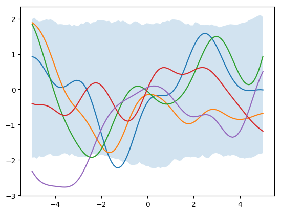
Next, let’s add in some observed data:
x_obs = np.array([-4.5, -3.5, -0.5, 0, 1])
y_obs = np.array([-2, 0, 1, 2, -1])
We now need to calculate the covariance between our unobserved data (x_star) and our observed data (x_obs), as well as the covariance among x_obs points as well. The first for loop calculates observed covariances. The second for loop calculates observed-new covariances.
N_obs = 5
K_obs = np.empty((N_obs, N_obs))
for i in range(N_obs):
	for j in range(N_obs):
		K_obs[i,j] = np.exp(-0.5 * (x_obs[i] - x_obs[j])**2)

K_obs_star = np.empty((N_obs, N_star))
for i in range(N_obs):
	for j in range(N_star):
		K_obs_star[i,j] = np.exp(-0.5*(x_obs[i] - x_star[j])**2)
We can then get our posterior distributions:
\( \boldsymbol{\mu} = \boldsymbol{K}_{obs}^{*’} \boldsymbol{K}_{obs}^{-1} \boldsymbol{y}_{obs} \)
\( \boldsymbol{\Sigma} = \boldsymbol{K}^{*} – \boldsymbol{K}_{obs}^{*’} \boldsymbol{K}_{obs}^{-1} \boldsymbol{K}_{obs}^{*} \)
and simulate from this posterior distribution.
post_mean = K_obs_star.T.dot(np.linalg.pinv(K_obs)).dot(y_obs)
post_var = K_star - K_obs_star.T.dot(np.linalg.pinv(K_obs)).dot(K_obs_star)

posteriors = st.multivariate_normal.rvs(mean=post_mean, cov=post_var, size=1000)

for i in range(1000):
	plt.plot(x_star, posteriors[i], c='k', alpha=0.01)

plt.plot(x_obs, y_obs, 'ro')
plt.show()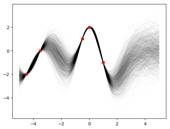
This may not look exactly like the Rasmussen and Williams Fig. 2.2b because I guessed at the data points and they may not be quite right. As the authors point out, we can actually plot what the covariance looks like for difference x-values, say \(x=-1,2,3\).
plt.plot(x_star, post_var[30], label='x= = -2')
plt.plot(x_star, post_var[60], label='x = 1')
plt.plot(x_star, post_var[80], label='x = 3')
plt.ylabel('Posterior Covariance')
plt.legend()
plt.show()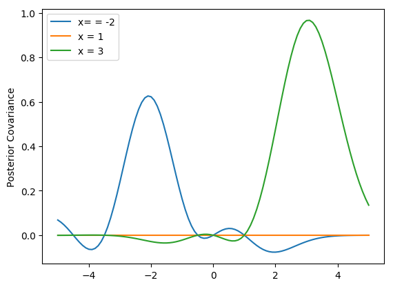
In this case, however, we’ve forced the scale to be equal to 1, that is you have to be at least one unit away on the x-axis before you begin to see large changes \(y\). We can incorporate a scale parameter \(\lambda\) to change that. We can use another parameter \(\sigma_f^2\) to control the noise in the signal (that is, how close to the points does the line have to pass) and we can add further noise by assuming measurement error \(\sigma_n^2\).
\(cov(x_i, x_j) = \sigma_f^2 \text{exp}[-\frac{1}{2\lambda^2} (x_i – x_j)^2] + \delta_{ij}\sigma_n^2\)Let’s make some new data:
x_obs = np.array([-7, -5.5, -5, -4.8, -3, -2.8, -1.5,
	-1, -0.5, 0.25, 0.5, 1, 2.5, 2.6, 4.5, 4.6, 5, 5.5, 6])
y_obs = np.array([-2, 0, 0.1, -1, -1.2, -1.15, 0.5, 1.5, 1.75,
	0, -0.9, -1, -2.5, -2, -1.5, -1, -1.5, -1.1, -1])
x_star = np.linspace(-7, 7, N_star)
Next, make a couple of functions to calculate \(\boldsymbol{K}_{obs}\), \(\boldsymbol{K}^{*}\), and \(\boldsymbol{K}_{obs}^{*}\).
def k_star(l, sf, sn, x_s):
	N_star = len(x_s)
	K_star = np.empty((N_star, N_star))
	for i in range(N_star):
		for j in range(N_star):
			K_star[i,j] = sf**2*np.exp(-(1.0 / (2.0*l**2)) * (x_s[i] - x_s[j])**2)
	return K_star

def k_obs(l, sf, sn, x_o):
	N_obs = len(x_o)
	K_obs = np.empty((N_obs, N_obs))
	for i in range(N_obs):
		for j in range(N_obs):
			K_obs[i,j] = sf**2*np.exp(-(1.0 / (2.0*l**2)) * (x_o[i] - x_o[j])**2)
	for i in range(N_obs):
		K_obs[i,i] += sn**2
	return K_obs

def k_obs_star(l, sf, sn, x_o, x_s):
	N_obs = len(x_o)
	N_star = len(x_s)
	K_obs_star = np.empty((N_obs, N_star))
	for i in range(N_obs):
		for j in range(N_star):
			K_obs_star[i,j] = sf**2*np.exp(-(1.0 / (2.0*l**2)) *(x_o[i] - x_s[j])**2)
	return K_obs_star
Then run the code for the various sets of parameters. Let’s start with (1, 1, 0.1):
K_star = k_star(1,1,0.2,x_star)
K_obs = k_obs(1,1,0.2, x_obs)
K_obs_star = k_obs_star(1,1,0.2,x_obs, x_star)

post_mean = K_obs_star.T.dot(np.linalg.pinv(K_obs)).dot(y_obs)
post_var = K_star - K_obs_star.T.dot(np.linalg.pinv(K_obs)).dot(K_obs_star)

posteriors = st.multivariate_normal.rvs(mean=post_mean, cov=post_var, size=1000)

for i in range(1000):
	plt.plot(x_star, posteriors[i], c='k', alpha=0.01)

plt.plot(x_star, posteriors.mean(axis=0))
plt.plot(x_obs, y_obs, 'ro')
plt.show()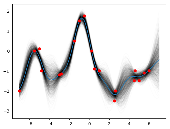
Then try (0.3, 1.08, 0.00005):
K_star = k_star(0.3, 1.08, 0.00005, x_star)
K_obs = k_obs(0.3, 1.08, 0.00005,  x_obs)
K_obs_star = k_obs_star(0.3, 1.08, 0.00005, x_obs, x_star)

post_mean = K_obs_star.T.dot(np.linalg.pinv(K_obs)).dot(y_obs)
post_var = K_star - K_obs_star.T.dot(np.linalg.pinv(K_obs)).dot(K_obs_star)

posteriors = st.multivariate_normal.rvs(mean=post_mean, cov=post_var, size=1000)

for i in range(1000):
	plt.plot(x_star, posteriors[i], c='k', alpha=0.01)

plt.plot(x_star, posteriors.mean(axis=0))

plt.plot(x_obs, y_obs, 'ro')
plt.show()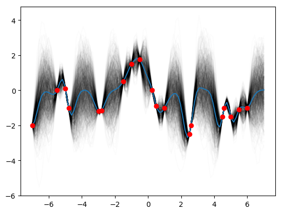
Then finally (3, 1.16, 0.89):
K_star = k_star(3, 1.16, 0.89, x_star)
K_obs = k_obs(3, 1.16, 0.89,  x_obs)
K_obs_star = k_obs_star(3, 1.16, 0.89, x_obs, x_star)

post_mean = K_obs_star.T.dot(np.linalg.pinv(K_obs)).dot(y_obs)
post_var = K_star - K_obs_star.T.dot(np.linalg.pinv(K_obs)).dot(K_obs_star)

posteriors = st.multivariate_normal.rvs(mean=post_mean, cov=post_var, size=1000)

for i in range(1000):
	plt.plot(x_star, posteriors[i], c='k', alpha=0.01)

plt.plot(x_star, posteriors.mean(axis=0))

plt.plot(x_obs, y_obs, 'ro')
plt.show()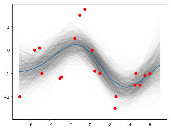
And there you have it! Figs 2.2, 2.4, and 2.5 from Rasmussen and Williams.