
Foliar A/Ci curves, which relate carbon biochemistry to photosynthesis rates, provide an extraordinary amount of information about plant physiology. While the methods for actually measuring A/Ci curves are well established (although new methods are being developed), the parameters can be notoriously difficult to estimate. A number of papers explain the best practices for doing so, so I figured I’d post my method (and the code) here.
A/Ci curves were described by Farquhar, von Caemmerer and Berry (hereon FvCB) as a means of estimating the mechanics of carbon fixation in plants. The model consists of two main parts (technically there’s three, but I’m going to ignore TPU for now since it is rarely estimated).
The first component describes CO2 fixation in terms of substrate limitation of Rubisco (i.e. CO2 limitation of Rubisco binding):
\( A_c = \frac{V_{cmax} (Ci – \Gamma^*)}{Ci + K_c (1 + \frac{O}{K_O})} \)where \(V_{cmax}\) is the maximum rate of Rubisco carboxylase activity, and \(K_c\), \(Ko\), \(\Gamma^*\)and O are fixed constants.
The second component describes CO2 fixation in terms of electron-transport limitation of RuBP regeneration:
\( A_j = \frac{J(Ci – \Gamma^*)}{4Ci + 8\Gamma^*} \)where J is the maximum rate of photosynthetic electron transport.
Thus, photosynthesis is determined by which of these two rates is limiting, minus a correction for metabolic respiration:
\(A = min\{A_c, A_j\} – Rd\)Estimating Vcmax, J, and Rd is often difficult for two reasons: 1) this is a non-linear equation, and those are tricky just be default, and 2) this is actually a changepoint function (as pointed out by Gu et al.). As Gu et al. point out, changepoint functions are difficult because parameter estimation of one function in the range where it isn’t limiting shouldn’t, but does, have an influence on parameter estimates of the other function.
As a result of these two problems, the FvCB model has a messy likelihood profile, completely full of local minima, wonky shapes, etc. Here’s the likelihood profile for Vcmax and J (assuming Rd = 1) for an A/Ci curve on smooth brome:
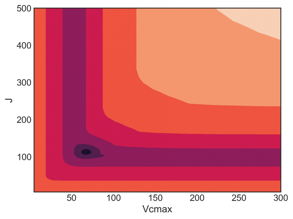
This isn’t great. A good profile would be concentric rings, where both parameters move towards a minimum. But there are lots of flat regions, where a gradient-based optimizer can get stuck. Look at the bottom of the graph at low J. Here’s a profile (slice) of that:
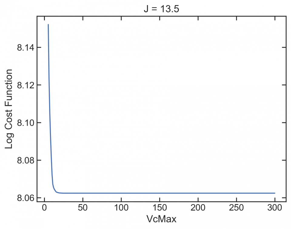
If the optimizer winds up here, it’s going to get stuck.
Gradient optimizers are favored because they are generally much faster than a grid search, but a grid search is basically the most reliable method to find the true global minimum. That’s why they were advocated by Dubois et al. 2007. But they are considered slow. For example, Dubois et al. did a grid search over 4,400 combinations of Vcmax, J, and Rd and it takes 14 seconds. Further, their grid was really coarse. Here’s how this might look in Python:
# read in data.
df = pd.read_csv('aci_test.csv')

# set up constants as from Dubois et al. (2007)
R = 0.008314
GammaStar = np.exp(19.02-38.83/(R*(25+273.15)))
Kc = np.exp(38.05-79.43/(R*(25+273.15)))
Ko = np.exp(20.30-36.38/(R*(25+273.15)))
O = 210

# extract the columns and turn them into arrays
ci = np.array(df['Ci'])
A = np.array(df['A'])

# make a grid of all possible combinations
# this grid contains 8000 combinations of Vcmax, J, Rd
VV, JJ, RR = np.meshgrid(np.linspace(5, 300, 20),
                         np.linspace(5, 500, 20),
                         np.linspace(-1, 10.1, 20))

# make an empty container to store results
res = np.empty(VV.shape)

# write a function that wraps around the for loop just for timing
def timing_wrap():
    for i in range(20):
        for j in range(20):
            for k in range(20):
                co2_lim = ( (VV[i,j,k]*(ci - GammaStar)) / (ci +(Kc*(1+(O/Ko)))) )
                rubp_lim = ((JJ[i,j,k]*(ci- GammaStar))/((4*ci)+(8*GammaStar)))
                Ahat = np.minimum(co2_lim, rubp_lim) - RR[i,j,k]
                err = A - Ahat
                res = np.sum(err**2)

%timeit timing_wrap()
173 ms ± 1.92 ms per loop (mean ± std. dev. of 7 runs, 10 loops each)
This for-loop over 8,000 parameters takes 0.173 seconds on my computer. If we bump up the number of combinations to 200,000 (100 points for Vcmax, 100 points for J, 20 for Rd), we get:
VV, JJ, RR = np.meshgrid(np.linspace(5, 300, 100),
                         np.linspace(5, 500, 100),
                         np.linspace(-1, 10.1, 20))

res = np.empty(VV.shape)
def timing_wrap():
    for i in range(100):
        for j in range(100):
            for k in range(20):
                co2_lim = ( (VV[i,j,k]*(ci - GammaStar)) / (ci +(Kc*(1+(O/Ko)))) )
                rubp_lim = ((JJ[i,j,k]*(ci- GammaStar))/((4*ci)+(8*GammaStar)))
                Ahat = np.minimum(co2_lim, rubp_lim) - RR[i,j,k]
                err = A - Ahat
                res = np.sum(err**2)

%timeit timing_wrap()
4.46 s ± 239 ms per loop (mean ± std. dev. of 7 runs, 1 loop each)
The time goes up exponentially as we make the grid finer and finer. What we would like to be able to do is search an incredibly fine grid very quickly. Fortunately, vectorization in numpy/Python makes this possible. It takes advantage of broadcasting arrays:
def timing_wrap():
    co2_lim = ( (VV[:,:,:,None]*(ci[None,None,None,:] - GammaStar)) / (ci[None,None,None,:] +(Kc*(1+(O/Ko)))) )
    rubp_lim = ((JJ[:,:,:,None]*(ci[None,None,None,:]- GammaStar))/((4*ci[None,None,None,:])+(8*GammaStar)))
    Ahat = np.minimum(co2_lim, rubp_lim) - RR[:,:,:,None]
    err = A[None,None,None,:] - Ahat
    sse = (err**2).sum(axis=-1)

%timeit timing_wrap()
43.9 ms ± 203 µs per loop (mean ± std. dev. of 7 runs, 10 loops each)
We can do the exact same thing as above, but without any for-loops. This 200,000 point grid runs in 0.4 seconds! Broadcasting enables us to search an incredibly find grid to get into the ball-park:
VV, JJ, RR = np.meshgrid(np.linspace(5, 300, 300),
                         np.linspace(5, 500, 300),
                         np.linspace(-1, 10.1, 30))


def timing_wrap():
    co2_lim = ( (VV[:,:,:,None]*(ci[None,None,None,:] - GammaStar)) / (ci[None,None,None,:] +(Kc*(1+(O/Ko)))) )
    rubp_lim = ((JJ[:,:,:,None]*(ci[None,None,None,:]- GammaStar))/((4*ci[None,None,None,:])+(8*GammaStar)))
    Ahat = np.minimum(co2_lim, rubp_lim) - RR[:,:,:,None]
    err = A[None,None,None,:] - Ahat
    sse = (err**2).sum(axis=-1)

%timeit timing_wrap()
633 ms ± 2.15 ms per loop (mean ± std. dev. of 7 runs, 1 loop each)
where we can search 2.7 million grid spaces in 0.6 seconds. Now we can get our best estimates:
res = timing_wrap()

# get the INDEX of the minimum
idx = np.unravel_index(res.argmin(), res.shape)

# extract parameters
Vcmax = VV[idx]
J = JJ[idx]
Rd = RR[idx]
print(Vcmax)
67.15719063545151
print(J)
112.6086956521739
print(Rd)
2.0620689655172413
If we want to go one step further, we can develop a STAN model that samples in this region, and we can use our best estimates to start the model in a region that is very likely at least close to the global minimum:
FvCB_mod = """
data{
    int N;
    vector[N] ci;
    vector[N] y;
}
transformed data{
    real R = 0.008314;
    real GammaStar = exp(19.02-38.83/(R*(25+273.15)));
    real Kc = exp(38.05-79.43/(R*(25+273.15)));
    real Ko = exp(20.30-36.38/(R*(25+273.15)));
    real O = 210;
}
parameters{
    real<lower=0> Vcmax;
    real<lower=0> J;
    real Rd;
    real<lower=0> sd_y;
}
transformed parameters{
    vector[N] co_lim;
    vector[N] rubp_lim;
    vector[N] yhat;

    for(n in 1:N){
        co_lim[n] = ((Vcmax*(ci[n]-GammaStar))/(ci[n]+(Kc*(1+(O/Ko)))));
        rubp_lim[n] = ((J*(ci[n]-GammaStar))/((4*ci[n])+(8*GammaStar)));
        yhat[n] = fmin(co_lim[n], rubp_lim[n]) - Rd;
    }
}
model{
    y ~ normal(yhat, sd_y);
}
"""
fvcb_comp = pyst.StanModel(model_code=FvCB_mod)

df_data = {'N': df.shape[0],
               'ci': df['Ci'],
               'y': df['A']}

init = {'Vcmax': Vcmax, 'J': J, 'Rd': Rd}

fvcb_opt = fvcb_comp.sampling(data=df_data, iter=50000, chains=1, init=[init])
The problem here is that the STAN sampler can still get stuck, but that’s OK. If it does, just re-run it and it sorts itself out.
arviz.plot_density(fvcb_opt, var_names=['Vcmax', 'J', 'Rd'])
plt.show()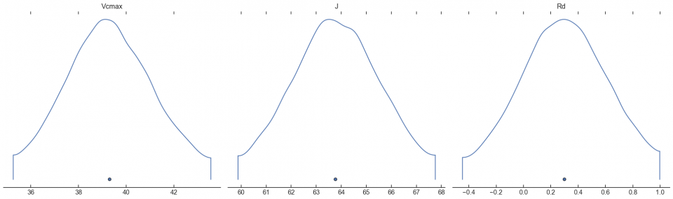
Personally, I always recommend following up the grid search with some kind of optimizer (nls, STAN, etc) using the grid parameters as initial guesses. To see why, look at the values of Rd. The grid search identified Rd = 2.1. But putting this into an optimizer came out with Rd = 0.3. Which of these is accurate, I can’t say. I need to do more work with simulated data to know which is more accurate. But for the time being, here is a highly efficient, non-gradient-based approach to estimating A/Ci parameters.