Even Faster Gaussian Processes in STAN Using functions

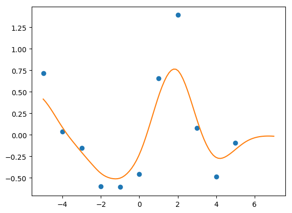
In my last post, I discussed how to get predictions from Gaussian Processes in STAN quickly using the analytical solution. I was able to get it down to 3.8 seconds, which is pretty quick. But I can do better.

One of this issues you may or may not have noticed is, using the model wherein posterior predictions are generated quantities, your computer bogs down with anything over 1000 iterations (I know mine froze up). The issue here is that generated quantities saves all the variables into memory, including those large matrices \( \boldsymbol{K}_{obs}, \boldsymbol{K}_{obs}^{*}, \boldsymbol{K}^{*} \) . We can resolve this issue, and speed things up, using functions to calculate the predictive values while storing the matrices only as local variables within the function (they are not saved in memory).

One obvious solution is to not calculate them within STAN, but to do it externally. Python can do this relatively quickly with judicious use of numpy (whose linear algebra functions are all written in C and so very fast) and numba/just-in-time compilers. However, since STAN compiles everything into C++,  and many of its linear algebra functions are optimized for speed, it makes sense to do it all in STAN. Fortunately, we can create our own functions within STAN to do this, which are then compiled and executed in C++. The code is as follows:

import numpy as np
import matplotlib.pyplot as plt
import pystan as pyst

X = np.arange(-5, 6)
Y_m = np.sin(X)
Y = Y_m + np.random.normal(0, 0.5, len(Y_m))

X_pred = np.linspace(-5, 7, 100)

gp_pred = """
functions{
	// radial basis, or square exponential, function
	matrix rbf(int Nx, vector x, int Ny, vector y, real eta, real rho){
		matrix[Nx,Ny] K;
		for(i in 1:Nx){
			for(j in 1:Ny){
				K[i,j] = eta*exp(-rho*pow(x[i]-y[j], 2));
			}
		}
		return K;
	}

        // all of the posterior calculations are now done within this function
	vector post_pred_rng(real eta, real rho, real sn, int No, vector xo, int Np, vector xp, vector yobs){
			matrix[No,No] Ko;
			matrix[Np,Np] Kp;
			matrix[No,Np] Kop;
			matrix[Np,No] Ko_inv_t;
			vector[Np] mu_p;
			matrix[Np,Np] Tau;
			matrix[Np,Np] L2;
			vector[Np] Yp;

                        // note the use of matrix multiplication for the sn noise, to remove any for-loops
			Ko = rbf(No, xo, No, xo, eta, rho) + diag_matrix(rep_vector(1, No))*sn ;
			Kp = rbf(Np, xp, Np, xp, eta, rho) + diag_matrix(rep_vector(1, Np))*sn ;
			Kop = rbf(No, xo, Np, xp, eta, rho) ;
			
			Ko_inv_t = Kop' / Ko;
			mu_p = Ko_inv_t * yobs;
			Tau = Kp - Ko_inv_t * Kop;
			L2 = cholesky_decompose(Tau);
			Yp = mu_p + L2*rep_vector(normal_rng(0,1), Np);
			return Yp;
	}
}
data{
	int<lower=1> N1;
	int<lower=1> N2;
	vector[N1] X;
	vector[N1] Y;
	vector[N2] Xp ;
}
transformed data{
	vector[N1] mu;
	for(n in 1:N1) mu[n] = 0;
}
parameters{
	real<lower=0> eta_sq;
	real<lower=0> inv_rho_sq;
	real<lower=0> sigma_sq;
}
transformed parameters{
	real<lower=0> rho_sq;
	rho_sq = inv(inv_rho_sq);
}
model{
	matrix[N1,N1] Sigma;
	matrix[N1,N1] L_S;

        // can actually use those functions here, too!!
	Sigma = rbf(N1, X, N1, X, eta_sq, rho_sq) + diag_matrix(rep_vector(1, N1))*sigma_sq;

	L_S = cholesky_decompose(Sigma);
	Y ~ multi_normal_cholesky(mu, L_S);

	eta_sq ~ cauchy(0,5);
	inv_rho_sq ~ cauchy(0,5);
	sigma_sq ~ cauchy(0, 5);
}
generated quantities{
	vector[N2] Ypred;
   
        // this is where the magic happens. note that now we only store Ypred,
        // instead of all those extraneous matrices
	Ypred = post_pred_rng(eta_sq, rho_sq, sigma_sq,
		N1, X, N2, Xp, Y);
}
"""

gp1 = pyst.StanModel(model_code=gp_pred)

data1 = {'N1': len(X), 'X': X, 'Y': Y, 'Xp': X_pred, 'N2': len(X_pred)}
fit_gp1 = gp1.sampling(data1, iter=1000)

There are a couple of tricks here. I used a diagonal matrix \(\boldsymbol{I}\sigma_n\) to remove a for-loop in calculating the noise variance.  It has the added benefit of cleaning up the code (I find for-loops to be messy to read, I like things tidy). Second, by using functions, the generated quantities only stores the predictions, not all the extra matrices, freeing up tons of memory. 

One other thing to note is that the prediction function ends with the suffix ‘_rng’. This is because it is a random number generator, drawing random observations from the posterior distribution. Using the ‘_rng’ suffix allows the function to access other ‘_rng’ functions, chiefly the normal_rng function which draws random normal deviates. That’s necessary for the cholesky trick to turn N(0,1) numbers into the posterior distribution (see the last post). However, normal_rng only returns ONE number, so you have to repeat it for however many observations you need, hence the rep_vector( ) wrapper.

This code is extremely fast. After compilation, it executes 4 chains, 1000 iterations in roughly 1 second (compared to just over three from the previous post). Further, since I no longer have memory issues, I can run more iterations. Whereas 5000 iterations froze my computer before, now it executes in 5 seconds. 10,000 iterations, previously unimaginable on my laptop, runs in 10 seconds.

Pretty great.