As described in an earlier post, Gaussian process models are a fast, flexible tool for making predictions. They’re relatively easy to program if you happen to know the parameters of your covariance function/kernel, but what if you want to estimate them from the data? There are several methods available, but my favorite so far is STAN. True, it requires programming the kernel by hand, but I actually find this easier to understand than trying to parse out the kernel functions from, say, scikit-learn.
STAN can fit GP models quickly, but there are certain tricks you can do that make it lightning fast and accurate. I’ve had trouble getting scikit to converge on a stable/accurate solution, but STAN does this with no problem. Plus, the Hamiltonian Monte-Carlo sampler is very quick for GPs (see the STAN User Manual for more).
Here’s a quick tutorial on how to fit GPs in STAN, and how to speed them up. First, let’s import our modules and simulate some fake data:
import numpy as np
import scipy.stats as st
import matplotlib.pyplot as plt

X = np.arange(-5, 6)
Y_m = np.sin(X)
Y = Y_m + np.random.normal(0, 0.5, len(Y_m))
Now, let’s develop the STAN model. Here’s the boilerplate model for a GP using a squared-exponential model (taken right from the STAN manual).
gp_no_pred = """
data{
	int<lower=1> N;
	vector[N] X;
	vector[N] Y;
}
transformed data{
	vector[N] mu;

	for(n in 1:N) mu[n] = 0;
}
parameters{
	real<lower=0> s_f;
	real<lower=0> inv_rho;
	real<lower=0> s_n;
}
transformed parameters{
	real<lower=0> rho;

	rho = inv(inv_rho);
}
model{
	matrix[N,N] Sigma;

	for(i in 1:(N-1)){
		for(j in (i+1):N){
			Sigma[i,j] = s_f * exp(-rho * pow(X[i]-X[j], 2));
                        Sigma[j,i] = Sigma[i,j];
		}
	}

	for(k in 1:N){
		Sigma[k,k] = s_f + s_n;
	}

	Y ~ multi_normal(mu, Sigma);
        s_f ~ cauchy(0,5);
        inv_rho ~ cauchy(0,5);
        s_n ~ cauchy(0,5);

}
"""
This model fits the parameters of the kernel. On my computer, it does so in about 0.15 seconds total (1000 iterations).
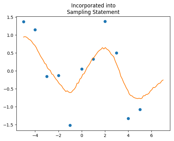
Now that we know what the hyperparameters are, we’d like to predict new values, but we also want to do so incorporating full uncertainty in the hyperparameters. The way the STAN manual says to go about this is to make a second vector containing the locations you’d like to predict, paste those together to the X values you have, make a vector of prediction points as parameters, paste those to the Y values you have, and feed those into the multivariate normal distribution as one big mush. The issue here is that the covariance matrix, Sigma, gets very large very fast. Large covariance matrices take a while to invert in the multivariate probability density, and so slows down the sampler.
Here’s the model, after making a vector of 100 prediction points to get a smooth line:
X_pred = np.linspace(-5, 7, 100)

gp_pred1 = """
data{
	int<lower=1> N1;
	int<lower=1> N2;
	vector[N1] X;
	vector[N1] Y;
	vector[N2] Xp;
}
transformed data{
	int<lower=1> N;
	vector[N1+N2] Xf;
	vector[N1+N2] mu;

	N = N1+N2;
	for(n in 1:N) mu[n] = 0;
	for(n in 1:N1) Xf[n] = X[n];
	for(n in 1:N2) Xf[N1+n] = Xp[n];
}
parameters{
	real<lower=0> s_f;
	real<lower=0> inv_rho;
	real<lower=0> s_n;
	vector[N2] Yp;
}
transformed parameters{
	real<lower=0> rho;

	rho = inv(inv_rho);
}
model{
	matrix[N,N] Sigma;
	vector[N] Yf;

	for(n in 1:N1) Yf[n] = Y[n];
	for(n in 1:N2) Yf[N1+n] = Yp[n];

	for(i in 1:(N-1)){
		for(j in (i+1):N){
			Sigma[i,j] = s_f * exp(-rho * pow(Xf[i]-Xf[j], 2));
			Sigma[j,i] = Sigma[i,j];
		}
	}

	for(k in 1:N){
		Sigma[k,k] = s_f + s_n;
	}

	Yf ~ multi_normal(mu, Sigma);

	s_f ~ cauchy(0,5);
	inv_rho ~ cauchy(0,5);
	s_n ~ cauchy(0, 5);
}
"""
This is extremely slow, taking about 81 seconds on my computer (up from less than one second). Taking the cholesky decompose of Sigma an using multi_normal_cholesky didn’t speed things up, either.
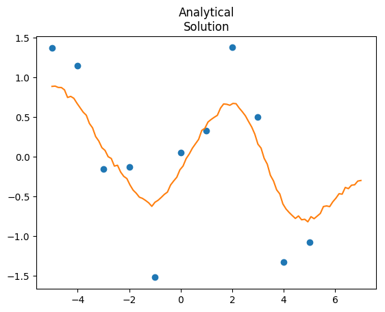
We can speed this up by taking advantage of the analytical form of the solution. That is, once we know the hyperparameters of the kernel from the observed data, we can directly calculate the multivariate normal distribution of the predicted data:
\( P(Y_p | X_p, X_o, Y_o) \sim Normal(\boldsymbol{K}_{obs}^{*’} \boldsymbol{K}_{obs}^{-1} \boldsymbol{y}_{obs}, \boldsymbol{K}^{*} – \boldsymbol{K}_{obs}^{*’} \boldsymbol{K}_{obs}^{-1} \boldsymbol{K}_{obs}^{*}) \)We can calculate those quantities directly within STAN. Then, as an added trick, we can take advantage of the Cholesky decomposition to generate random samples of \( Y_p \) within STAN as well. Here’s the annotated model:
data{
	int<lower=1> N1;
	int<lower=1> N2;
	vector[N1] X;
	vector[N1] Y;
	vector[N2] Xp;
}
transformed data{
	vector[N1] mu;

	for(n in 1:N1) mu[n] = 0;
}
parameters{
	real<lower=0> s_f;
	real<lower=0> inv_rho;
	real<lower=0> s_n;
	// This is going to be just a generic (0,1) vector
	// for use in generating random samples
	vector[N2] z;
}
transformed parameters{
	real<lower=0> rho;

	rho = inv(inv_rho);
}
model{
	// kernel for only the observed data
	matrix[N1,N1] Sigma;

	for(i in 1:(N1-1)){
		for(j in (i+1):N1){
			Sigma[i,j] = s_f * exp(-rho * pow(X[i]-X[j], 2));
			Sigma[j,i] = Sigma[i,j];
		}
	}

	for(k in 1:N1){
		Sigma[k,k] = s_f + s_n;
	}

	// sampling statement for only the observed data
	Y ~ multi_normal(mu, Sigma);
	// generic sampling statement for z
	z ~ normal(0,1);

	s_f ~ cauchy(0,5);
	inv_rho ~ cauchy(0,5);
	s_n ~ cauchy(0, 5);
}
generated quantities{
	matrix[N1,N1] Ko;
	matrix[N2,N2] Kp;
	matrix[N1,N2] Kop;
	matrix[N1,N1] L;
	matrix[N1, N1] Ko_inv;
	vector[N2] mu_p;
	matrix[N2,N2] Tau;
	vector[N2] Yp;
	matrix[N2,N2] L2;

	// kernel for observed data
	for(i in 1:(N1-1)){
		for(j in (i+1):N1){
			Ko[i,j] = s_f * exp(-rho * pow(X[i]-X[j], 2));
			Ko[j,i] = Ko[i,j];
		}
	}

	for(k in 1:N1){
		Ko[k,k] = s_f + s_n;
	}

	// kernel for prediction data
	for(i in 1:(N2-1)){
		for(j in (i+1):N2){
			Kp[i,j] = s_f * exp(-rho * pow(Xp[i]-Xp[j], 2));
			Kp[j,i] = Kp[i,j];
		}
	}

	for(k in 1:N2){
		Kp[k,k] = s_f + s_n;
	}

	// kernel for observed-prediction cross
	for(i in 1:N1){
		for(j in 1:N2){
			Kop[i,j] = s_f * exp(-rho * pow(X[i]-Xp[j], 2));
		}
	}

	// Follow the algorithm 2.1 of Rassmussen and Williams
	// cholesky decompose Ko
	L = cholesky_decompose(Ko);
	Ko_inv = inverse(L') * inverse(L);
	// calculate the mean of the Y prediction
	mu_p = Kop' * Ko_inv * Y;
	// calculate the covariance of the Y prediction
	Tau = Kp - Kop' * Ko_inv * Kop;

	// Generate random samples from N(mu,Tau)
	L2 = cholesky_decompose(Tau);
	Yp = mu_p + L2*z;

}
"""
This model runs at 3.5 seconds, huge improvement over 81. If you want the predictions, just extract Yp, and that gives you predictions with full uncertainty. We can also compare the two outputs:
Note: I have no idea why, but upping the iterations from 1000 to 5000 causes the analytical solution model to freeze my computer. I can’t quite figure that one out.
Why are you adding s_n to s_f, instead of Sigma[k, k] in this line of code: for(k in 1:N1){
Sigma[k,k] = s_f + s_n;
}
?
The Rasmmussen and Williams textbook says that you add noise to the diagonal of the covariance matrix, which in this case is Sigma.
Have a look at the STAN manual. When I wrote this code, STAN didn’t have the cov_exp_quad function. In STAN, you can now code Sigma as
for i in 1:N
for j in 1:N
Sigma[i,j] = cov_exp_quad(x,s_f,rho)
for i in 1:N
Sigma[i,i] = Sigma[i,i] + s_n
This is basically the same thing because along the diagonals, cov_exp_quad reduces to s_f, so the diagonals are s_f + s_n.
I am new to STAN and in particular pystan. I have run the schools example in the pystan documentation and would like to understand how to run your examples in pystan. In particular, I want to understand how to see the values of the hyperparameters. Here is what I have so far:
X = np.arange(-5, 6)
Y_m = np.sin(X)
Y = Y_m + np.random.normal(0, 0.5, len(Y_m))
sm = pystan.StanModel(model_code=gp_no_pred)
gauss_dat = {‘N’: len(Y),
‘Y’: Y,
‘X’: X}
fit = sm.sampling(data=gauss_dat, iter=1000, chains=4, n_jobs=1)
print (fit)
How do I see the “best” mean and sigma?
If by ‘best’ you mean “most likely”, you need to extract the posteriors of the parameters. In the Gaussian Process case, the parameters are the length-scale (rho), process error (s_f), and observation error (s_n). You can extract the posteriors into a dataframe:
posteriors = pd.DataFrame(fit.extract([‘rho’, ‘s_f’, ‘s_n’]))
and now each column contains all posteriors estimates of the parameters. You can get the ‘best’ parameters by taking the mean or the median, generate confidence intervals, SEs, and basically whatever else you need to do.
You don’t have to extract into a DataFrame, if you run
posteriors = fit.extract([‘rho’, ‘s_f’, ‘s_n’])[[‘rho’, ‘s_f’, ‘s_n’]]
you’ll get a numpy array of the same format (column for each parameter). I just prefer DataFrames because generating summaries of parameters is easier and the column names help me remember what is what.
Can you also please share the code oh plotting the generated data ? shown in the two plots ?
thanks,